
Topographic profiles in python
Published:
Welcome to this blog post where we’ll explore how to plot topographic profiles from GPX tracks using Python. GPX tracks are a common format for storing GPS data, and they can be used to record a wide range of outdoor activities such as hiking, cycling, and running. You can use your favorite sports app to generate GPX data, Outdooractive, Openrunner…
One useful feature of GPX tracks is that they include elevation data, which allows us to create topographic profiles of the route. In this example, the data is my path along the Tour du Queyras trek, in the French Alps. The track can be downloaded here. Let’s get started!
import matplotlib.pyplot as plt
from xml.dom import minidom
import math

tracks = open('queyras.gpx')
xmldoc = minidom.parse(tracks)
track = xmldoc.getElementsByTagName('trkpt')
elevation = xmldoc.getElementsByTagName('ele')
datetime = xmldoc.getElementsByTagName('time')
n_track=len(track)

# Parse the GPX

lon_list=[] #longitudes
lat_list=[] #lattitutes
h_list=[] #heights
time_list=[] #timepoints
for s in range(n_track):
    lon,lat=track[s].attributes['lon'].value,track[s].attributes['lat'].value
    elev=elevation[s].firstChild.nodeValue

    # store lon,lat,elev
    lon_list.append(float(lon))
    lat_list.append(float(lat))
    h_list.append(float(elev))

    # extract timepoint in seconds
    dt=datetime[s].firstChild.nodeValue
    time_split=dt.split('T')
    hms_split=time_split[1].split(':')
    time_hour=int(hms_split[0])
    time_minute=int(hms_split[1])
    time_second=int(hms_split[2].split('Z')[0])
    total_second=time_hour*3600+time_minute*60+time_second
    time_list.append(total_second)

print(f"For point 0; longitude: {lon_list[0]}; lattitude: {lat_list[0]}; elevation: {h_list[0]}")
For point 0; longitude: 6.77668; lattitude: 44.67127; elevation: 1676.0
Seems like too much info? All we do is to parse the queyras.gpx file, which contains a bunch of bunch of points (track points, elevation and time stamps as obscure XML elements). We loop through all of those elemnts to extract lattitude/longitude geodetic coordinates, the elevation and the time stamp that we convert to seconds. Now we need some functions to work in cartesian coordinates and measure distance from the origin along the route:
# geodetic to cartesian
def geo2cart(lon,lat,h):
    # elliptic axes for Earth
    a=6378137 # WGS-84 major axis
    b=6356752.3142 # WGS-84 minor axis
    e2=1-(b**2/a**2)
    N=float(a/math.sqrt(1-e2*(math.sin(math.radians(abs(lat)))**2)))
    X=(N+h)*math.cos(math.radians(lat))*math.cos(math.radians(lon))
    Y=(N+h)*math.cos(math.radians(lat))*math.sin(math.radians(lon))
    return X,Y

def distance(x1,y1,x2,y2):
    d=math.sqrt((x1-x2)**2+(y1-y2)**2)
    return d
# populate distance list
d_list=[0.0]

l=0
for k in range(n_track-1):
    if k<(n_track-1):
        l=k+1
    else:
        l=k

    XY0=geo2cart(lon_list[k],lat_list[k],h_list[k])
    XY1=geo2cart(lon_list[l],lat_list[l],h_list[l])

    #DISTANCE
    d=distance(XY0[0],XY0[1],XY1[0],XY1[1])
    sum_d=d+d_list[-1]
    d_list.append(sum_d)
We are now ready to plot a topographic profile, from the distance to origin and altitude information. If we want a stylized version, ready to be imported on a travel blog:
import matplotlib as mpl

mpl.rcParams['axes.spines.right'] = False
mpl.rcParams['axes.spines.top'] = False
mpl.rcParams['axes.spines.left'] = False
mpl.rcParams['axes.spines.bottom'] = False


plt.figure(figsize=(20,2))
plt.plot(d_list,h_list,linewidth=5,c='k')
plt.ylim(1000,3000)
plt.xticks([])
plt.yticks([])
plt.savefig("profile.png",dpi=300)
plt.show()
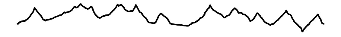
This is it, with this little tutorial you can generate a topographic profile in python from a GPX file.